Additive zoom level decomposition for e-profile Part III
Tweaking the quadtree algorithm for zoom level deconposition
Additive zoom level decomposition for e-profile Part III
Update! This algorithm does not work as good as expexted. Please skip to article IV.
In the former parts of this series I specified the two goals of the algorithm we are after:
- We need a 2^N decomposition to get additive zoom levels
- A certain tweak to allign the data points in each level optimal
In this part I like to dive into the second goal.
We do not know the data we will get for our vizualization as good as we would like. That is not a problem with the dataprocessing but lies in the nature of dealing with real world data. A certain measuerement system may deliver its data in 5 minute averages, but there may be an offset due to a restart of the device that shifts all following datapoints by a minute.
So we have to deal with data on an arbitrary grid in time as well as in altitude.
Here we have four points to assign to zoom levels.

A normal Quadtree decomposition will end up with.
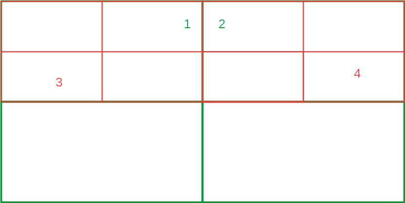
The first points (1,2) to assign to the quad tree will be on the top level grid.
But this is not what we want for our zoom levels. We would like to see the follwing:
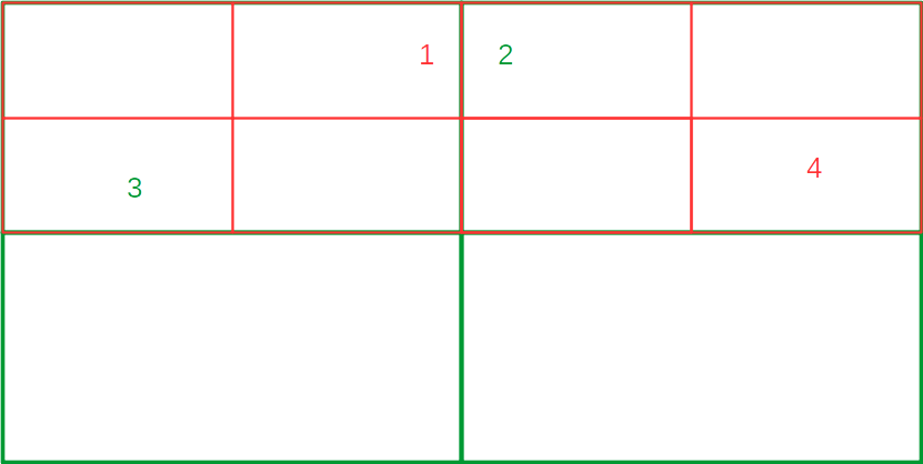
Our modified algorithm works as follows:
If a new datapoint enters a quadtree node and there is already a datapoint located, then the datapoints were conpared in terms of their location. The datapoint more left,down is chosen to stay on the current level. The other datapoint is send into the further area decomposition.
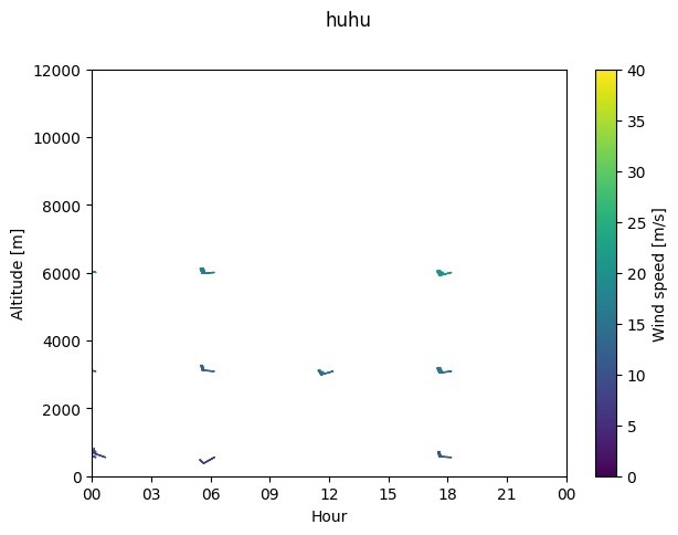
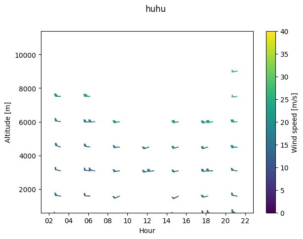
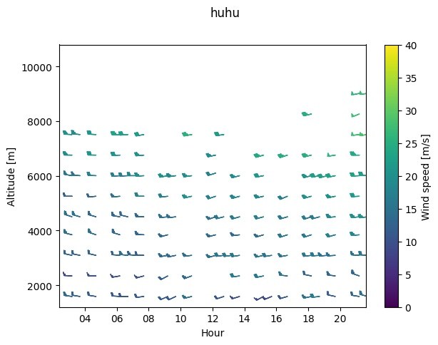
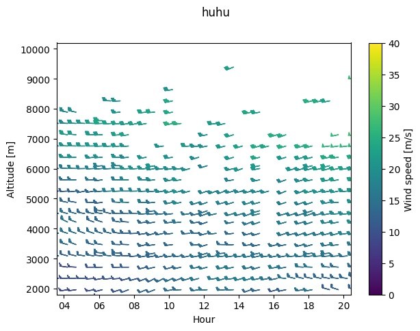
Here a preview of the results. Shown is the additve overlay of windbarbs according to their zoom-levels.
